I frequently find myself having to deal with identical data in spreadsheet rows. In this article, I’ll show you how to quickly delete duplicate rows in Excel.

How To Delete Duplicate Rows in Excel

I’ll show you three ways to remove duplicate rows in Excel spreadsheets. The first method is very easy and quick.

The second method takes slightly longer but is still simple. It involves a more hands-on approach to removing duplicate rows. The third method may take slightly longer and is a bit more involved.

Delete duplicate rows in Excel automatically

Excel has a feature that can automatically delete duplicates.

• Open the spreadsheet that contains the duplicate data.
• Open the Data tab.
• Click the Remove Duplicates button.
• A small options panel will open. Only if your spreadsheet has headers at the top of each row, check the box beside My list has headers. Do not check the box if your sheet does not use the top row for column headers.
• Click the OK button. 

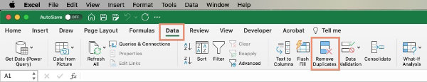
All duplicate rows should now be removed from your spreadsheet.

Use conditional formatting to find and delete duplicate rows manually

Depending on the complexity of your spreadsheet, you may be able to use a visual approach to removing the duplicates.

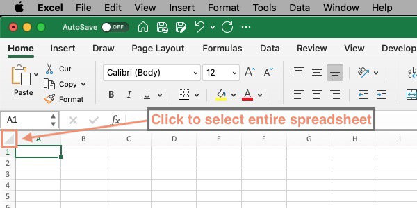
With your spreadsheet open, select the portion of the spreadsheet that contains duplicates. If you are searching the entire spreadsheet for duplicates, you can quickly select the entire spreadsheet by clicking the select all button at the top-left of the spreadsheet.

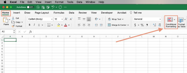
To mark duplicates in the spreadsheet:

• Open the Home tab.
• In the Styles group, click on Conditional Formatting.
  
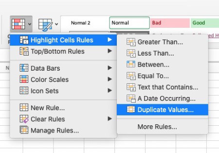
• Mouse over Highlight Cells Rules, then click Duplicate Values... from the sub-menu.
  
• In the New Formatting Rule panel, be sure Classic is set in the Style box.
• Format only unique or duplicate values should be selected in the second box. Click on the box and select it if it is not already set..
  
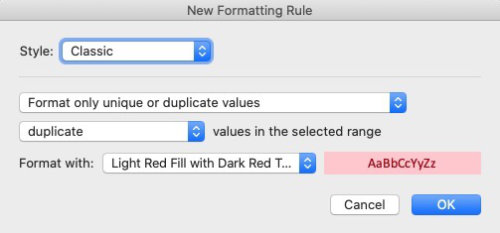
• Choose Duplicates in the third box, labeled Values in selected range.
• In the fourth box, labeled Format with, choose a color. Light red fill with dark red text will probably be pre-selected. Choose another from the list if you wish.
• Click OK.

Your duplicates should now be highlighted.

To delete the duplicate rows, I suggest leaving the first of the duplicate rows intact as the original. Then select the first duplicate by clicking the row number all the way to the left of the first column. 

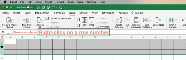
Hold the shift key and select the last duplicate row number.

All of the duplicate rows should be selected. To delete them, right-click a selected row number and click Delete.

Manually sort the data to find duplicate rows

Let’s say you have a spreadsheet with a few columns and perhaps fifty rows.

• Open your spreadsheet and click to open the Data tab.
• Place your cursor in the column that contains the potential duplicate data. In my case, I click into a column holding text.
• On the Data tab, click the Sort button.

If you have selected only one cell or a portion of your spreadsheet, you will see a Sort warning that gives you two options. You can expand the selection so that the entire spreadsheet will be sorted. 

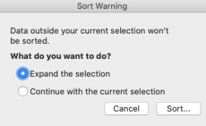
The other option is to sort only the selected area. If you have one column selected and choose to sort that column only, the rest of the columns in your spreadsheet will stay as they are and will no longer be synced with the first column. 

That may not be what you want. If it isn’t, either choose the option to expand the sort selection to include the entire spreadsheet or select an area of the spreadsheet that includes all of the data that you want to sort. To select your sort area, click in the top left corner of the area you want to sort and drag to the lower right corner so that your data stays synced during the sort.

If the first row of your spreadsheet is a header row, check the box near the top right corner of the Sort panel labeled My list has headers.

Warning: If your spreadsheet includes headers and you do not check that box indicating that your list has headers, the header row can be sorted along with your data. Checking the box leaves your header row intact and sorts the rows below the headers.

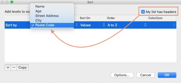
You’ll have to tell Excel how you want to sort the data. The Sort panel has several columns with options that allow you to customize your sort.

You will see headings above the columns labeled Column, Sort On, Order, and Color/Icon.

In my case, my spreadsheet contains a column with a header called Titles. I want to sort according to the titles, so I choose Title under Column.

Excel gives us the option to sort by the values that are in the cells, the cell color, the font color, or the cell icon. I chose Values because I want to sort the titles that are in the column alphabetically.

Under Order, I chose A to Z. If the content in the column that you are sorting is text, you’ll be given the option of sorting from A to Z or Z to A. 

If the content is populated with numbers such as currency, you’ll have the choice of Ascending or Descending. Other columns will be sorted as numbers if they are populated with numbers such Zip Codes (America’s postal codes), ages, etc..

Dates in the Sort by column will give you the option to sort by Oldest to newest or Newest to oldest.

After you set the sort options, click the OK button. Your data should now be sorted according to the settings you made.

Once you’ve sorted your data, you can look down the column that you sorted by and look for cells that contain identical information. Check that each of those rows contains identical data across all columns.

When you’ve found your duplicate rows, you can use the method described earlier to delete them.

Keeping it simple

The methods you learned above will work in a majority of situations that are similar to the scenarios mentioned. I recommend you start with the automatic method if your data is not too complex.

Add rows and columns in Microsoft Excel.

You’ll find more general Excel information in Microsoft’s official Excel documentation.