Setting up Excel spreadsheets with all the necessary formatting every time you need it can be time-consuming. In this article, you’ll learn some quick and easy ways to copy formatting in Excel for Windows and MacOS. 

You’ll be able to copy formatting from and to cells, rows, or columns within a sheet as well as between sheets and workbooks. 

How to copy formatting in Excel

Copying formatting in Excel is really as simple as copying and pasting. If you can do that, you’re already halfway there.

In the following tutorial, you’ll first learn to use Excel’s Autofill feature. You’ll learn to use Excel’s Format Painter. Then you’ll learn to copy formatting using the right-click menu and the toolbar.

The process is not difficult but there is a lot of information in this article. You can use the Navigation panel above to go straight to each of the individual methods.

Copy Excel formatting from one or more cells to connecting cells in the same rows or columns

One of the most common situations for copying formatting in Excel is to repeat one cell’s formatting to a group of connected cells in the same column or row.

One fast way to do that is to use the Autofill handle – the small square that appears in the lower right corner of the origin cell when it is selected.

To Autofill formatting in Excel for Windows:

• Select the cell that contains the formatting that you wish you to copy.
• Drag the Autofill handle across or down to select your target cells.
• Release the Autofill handle. 
• Click on the small settings box at the corner of your selection.
  
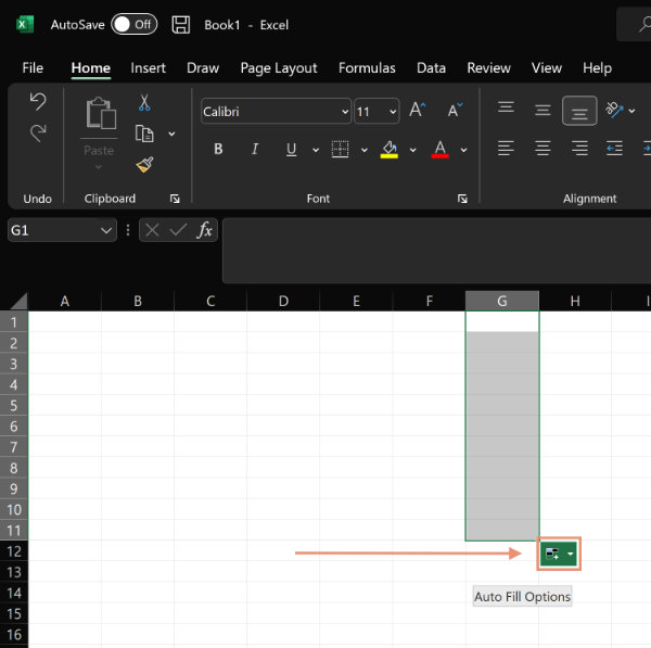
• In the Autofill options panel that opens, choose Fill formatting only.

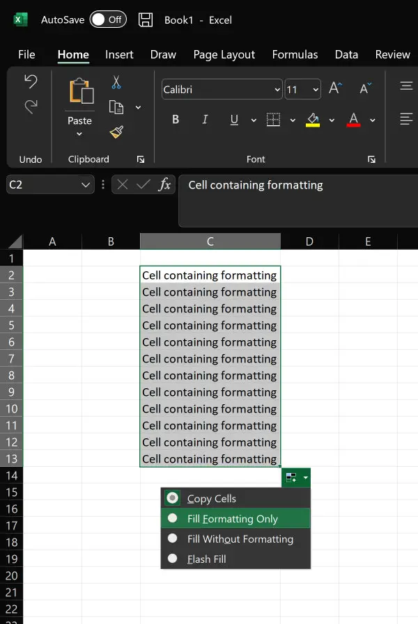
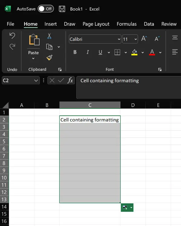
The cells in the dragged area will contain whatever was in the original cell, including text, until you choose Fill formatting only. Then, the text will remain in the original cell (if it contained text) and only the formatting will be copied to the target cells.

To Autofill formatting in Excel for Macs:

• Select the cell that contains the formatting that you wish you to copy.
• Right-click the Autofill handle and hold it while you drag it to select the target cells that you want to format.
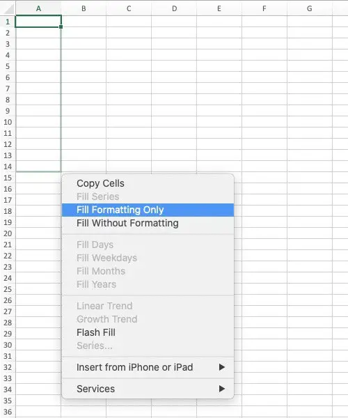
• Release the mouse to display a small submenu.
• Choose Fill formatting. 

Autofill formatting to multiple rows and columns in Excel

You can also copy the formatting of one cell to a range of cells that covers multiple rows down and multiple columns across. However, you’ll have to do the copying in two steps.

Use the process above for Autofilling the formatting down to as many rows as you need. Then repeat the process by dragging the handle across as many columns as you need. 

Autofill can only be used to copy formatting to adjacent cells. Therefore, it is no help if you need to copy formatting to non-adjacent cells such as across sheets or workbooks.

Autofill multiple formats in a row or column to adjacent rows or columns

The previous method allowed you to copy the formatting of one cell to a range of cells across and down a spreadsheet.

You can also copy formatting in a range of cells across a row or down a column to adjacent rows or columns.

This method can come in handy if you have a row of cells that contains different formatting in each cell across the row.

To copy varied formatting from a row of cells to multiple rows below or above the origin cells, do the following.

To Autofill formatting for a horizontal range of cells in a row in Excel for Windows:

• Select the range of cells that contains the formatting that you wish to copy.
• Drag the Autofill handle down as many rows as you need.
• Release the Autofill handle. 
• Click on the small settings box at the corner of your selection.
• In the Autofill options panel that opens, choose Fill formatting.

Use the same method to copy a vertical range of cells in columns across to other columns. The process is identical except you are copying across columns.

To Autofill formatting for a horizontal range of cells in a row in Excel for MacOS:

• Select the range of cells that contains the formatting that you wish to copy.
• Right-click on the Autofill handle and hold while you drag it down as many rows as you need. 
• Release the mouse to display a small submenu.
• Choose Fill formatting. 

Use the same method to copy a vertical range of cells in columns across to other columns. The process is identical except you are copying across columns.

Copy formatting between cells on a single Excel spreadsheet using the Format button

You can copy formatting from a single cell or a range of cells. 

The target cells can be adjacent or non-adjacent.

For example, you could copy the bold, italics, number format, etc. of one cell to another cell. The target cell would then have the same formatting as the origin cell. 

As another example, let’s say you have four columns with different formatting in each column. You can select those four columns and copy the formatting from them to columns in the same sheet or a different one. 

Each of the four target columns would take on the same formatting as the origin columns.

Follow these steps using the Format button to copy from a single cell to another cell in the same sheet.

• Click in the cell that contains the formatting that you want to copy.
• Open the Home tab.
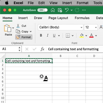
• Click the Format button in the Clipboard group under the Home tab. The cursor will change to a paintbrush.
  
• Click in the cell where you want to paste the formatting.
• Release the mouse button to paste the formatting into that cell. 

If you want to copy to multiple cells in a single column, click in the top or bottom cell of the target range and drag the paintbrush up or down to select all of the intended cells. Release the mouse to paste.

You can use the same technique to copy formatting to multiple cells in a row. After you’ve copied the formatting, click the first cell of the intended target and drag across until you’ve selected all the necessary cells. Release the mouse to paste the formatting.

You can also select a large range of target cells by placing the Format paintbrush cursor in the top left corner of the range. Then, drag across and down until you have selected the block of cells that you want to have the new formatting.

Copying formatting to non-adjacent cells

To select multiple non-adjacent cells or ranges of cells, click in the cell or range of cells whose formatting you want to copy. Then double-click the Format button before you click in any of the target cells.

After double-clicking the Format button, you would select the first target cell or range of cells with the Target paintbrush. Move on to the next cell or range of cells. 

Repeat until you are finished. 

Use the Escape key on your keyboard to stop the copy process.

A note of caution: When you click in the target cells with the Format paintbrush cursor, any existing formatting in those cells will be replaced by the formatting from the origin cell. For example, if the target cells were already formatted with bold text and a currency such as U.S. dollars, that formatting will go away unless the origin cell’s formatting also includes bold text and currency for U.S. dollars.

Copy Excel formatting from row to row

A single row in Excel can theoretically contain up to 16,384 cells. That is a world full of cells to format if you were to format them separately.

You can easily copy the formatting of one row to another row or a range of rows using either of the following methods.

Method one:

These instructions involve right-clicking with your mouse. If you’d like to use your mouse less, see the instructions later in this article for using the toolbar to copy and paste formatting.**

• Select the row number of the row whose formatting you want to copy in the number column on the left side.
• Right-click on the row number and select Copy (or use Control + C on Windows or Command + C on Macs).
• Open the Home tab and click the Format button in the first (Clipboard) section.
• With the Paintbrush cursor, select the row number of the target row where you want to paste the formatting.

Your target row should now display the formatting you copied from the origin row.

Remember to double-click the Format button before pasting if you intend to copy the formatting to multiple non-adjacent rows.

Method two:

• Click the row number on the far left to select the entire row.
• Right-click on the row number and select Copy (or use Control + C on Windows or Command + C on Macs).
• Go to the target row and select it by clicking its row number.
• Right-click on the target row number.
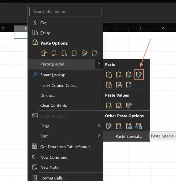
• Select Paste Special from the right-click menu.
• Select Formatting from the sub-menu.

The entire target row should now have the formatting of the origin row.

To paste the formatting to multiple non-consecutive rows, hold the Control key on Windows or the Command key on Macs as you right-click the intended target rows.

If the target row has more cells than the origin row, the formatting will be repeated until the last cell has been formatted. 

This could have unintended consequences if some cells in the row are formatted differently. The second set of columns may not have the intended formatting in all cells.

Copy formatting from column to column

A single column in Excel can contain 1,048,576 rows (assuming your computer’s hardware can handle that much processing).

The same two methods we applied to rows in the previous section work when copying Excel formatting from column to column.

Method one:

• Open the Home tab and click the Format button in the Clipboard section.
• Select the letter identifier at the top of the column whose formatting you want to copy.
• With the Paintbrush cursor, select the column identifier or letter of the target column where you want to paste the formatting.

Your target column should now display the formatting you copied from the origin column.

Method two: 

Click the Column letter (identifier) at the top to select the entire column.

• Right-click on the Column identifier (letter).
• Select Copy (or use Control + C on Windows or Command + C on Macs).
• Go to the target row and select it by clicking its row number.
• Right-click on the target number.
• Select Paste Special from the right-click menu.
• Select Formatting from the sub-menu.

The entire target column should now have the formatting of the origin column. 

To paste the formatting to multiple non-consecutive columns, hold the Control key on Windows or the Command key on Macs as you right-click to select the intended target columns.

Just as it is with rows, if the target column has more cells than the origin column, the formatting will be repeated until the last cell has been formatted.

Copy formatting between sheets in an Excel workbook

You can copy row or column formatting from one sheet in a workbook to a different sheet in the same workbook.

Use the same techniques given above. Just copy the formatting from the origin sheet. Then click the tab to open the target sheet. 

Use the same methods given above to paste the formatting into the other sheet.

Copy formatting between Excel workbooks

Open the Excel workbook and sheet that contains the formatting that you want to copy.

• Click the Column letter at the top or row number on the left to select the entire column or row.
• Right-click on the Column letter or row number.
• Select Copy (or use Control + C on Windows or Command + C on Macs).

Open the workbook and sheet to which you want to copy the formatting.

Go to the target column or row and select it by clicking its column letter or row number.

• Right-click on the target column letter or row number.
• Select Paste Special from the right-click menu.
• Select Formatting from the sub-menu.

The entire target column or row should now have the formatting of the origin column or row.

Copy formatting with formulas

You can copy the formatting and formulas from one Excel row or column to another.

• Click the row number or column letter to select the entire row or column that contains the formatting and formulas that you want to copy.
• Right-click on the row number or column letter.
• Select Copy (or use Control + C on Windows or Command + C on Macs).
• Go to the target row or column and select it by clicking its row number or column letter.
• Right-click on the target row number or column letter.
• Select Paste Special from the right-click menu.
• Select Formulas and number formatting from the sub-menu.

The entire target row or column should now have the formatting and formulas of the origin row or column.

Copy and paste formatting in Excel using toolbar buttons

**If using a mouse repeatedly is difficult for you, or if you have a computer with a touch-screen display, there is an alternative to the right-click menu options.

The following applies to most situations written in this article where the instructions tell you to right-click on a cell to copy or perform other actions.

You’ll still have to select the origin cells that contain the formatting that you want to copy. You can click or tap in the cells to select them.

From there, you’ll use the copy and paste tools in the Clipboard group under the Home tab. The Clipboard group is normally the first group on the left.

Where the instructions say to right-click and copy, you can click or tap the Copy button in the toolbar.

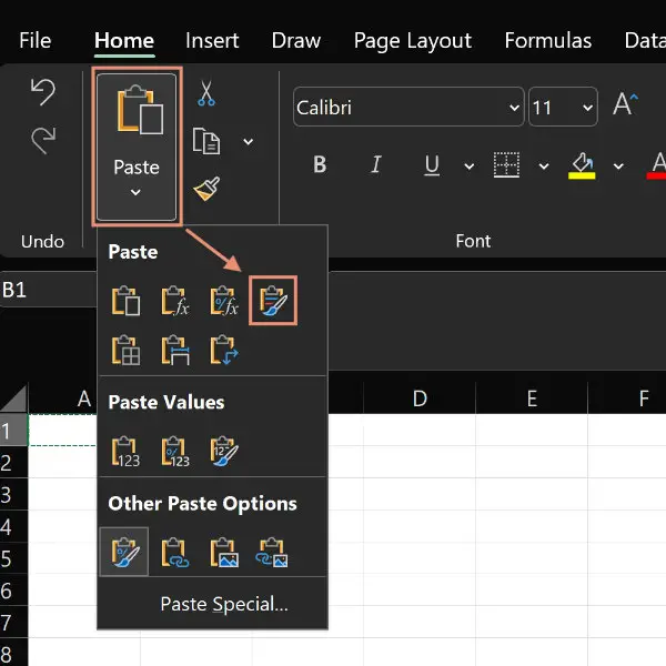
Where the instructions say to right-click and click Paste Special, you will instead click or tap the Paste button in Windows or the small arrow on the right side of the Paste button in Macs. 

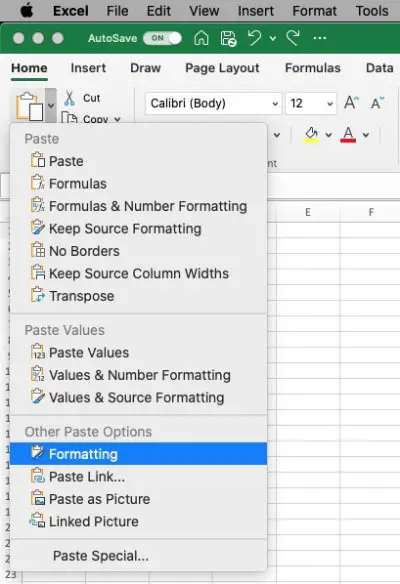
Note: If you only click on the button where the word Paste is in Excel for Macs, you will paste in content, formatting, and formulas. To control what you paste in, you must click or tap the small arrow on the right side of the button. That causes the same menu to pop up that you would see when you right-click and choose Paste Special.

In Excel for Macs, you’ll see the actual Paste Special menu with words. Click or tap Formatting. 

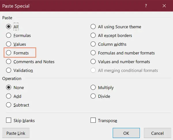
In Excel for Windows, you’ll see the Paste Special menu mostly with buttons. Under the words Paste Options there is a Formatting button.

In Excel for both Windows and Macs, if you click or tap Paste Special from the bottom of that menu, you’ll open a panel that shows all of the paste options. 

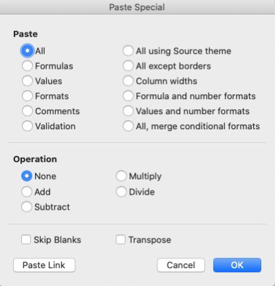
You’ll see more than one option in that panel relating to formatting. Choose Formats to paste only the formatting from the cell that you copied earlier.

Copy Excel formatting without content

You can copy formatting to a blank worksheet so that it will be ready and formatted when you add data to it.

Just use one of the techniques described above to copy formatting from a worksheet that contains data to a new blank worksheet.

When you type or paste in your unformatted data, you should see that it is now formatted like the worksheet you copied the formatting from.

Copy formatting (and formulas) for an entire worksheet in Excel

To copy formatting for an entire worksheet in Excel, open the worksheet that contains the formatting that you want to copy.

Click the button at the top of the number column (and left of the row letters). That should select your entire worksheet.

Right-click the same button and choose Copy (or use Control + C on Windows or Command + C on Macs).

Go to your new blank worksheet and click the button to select the entire worksheet.

Right-click the button and choose Paste Special…. Select Formatting. Select Formulas and number formatting if you want to include formulas.

Potential issues after copying conditional formatting in Excel

Some conditional formatting is copied when you use the methods we’ve already discussed.

It is possible that you may come across a cell reference that is incorrect, causing your conditional formatting to be off in places. If that happens, you can open the conditional formatting settings and correct the error.

You’ll find Conditional Formatting in the Styles group under the Home tab.

• Click the Conditional Formatting button.
• Choose Manage Rules.
• Find and select the rule that seems to be misbehaving.
• Click the Edit rule button at the bottom of the window and correct the cell references.

The following article may also be useful:

How to add rows and columns in Microsoft Excel.

Microsoft’s official Excel documentation