Excel gives us ways to format sheets so that our data is easier to organize and read. If you are visually challenged, your formatting may start with making the gridlines in Excel more visible. I’ll show you two ways to make the lines between cells easier to see.

I’ll also show you how to create a custom style that quickly pops in bolder cell borders.

How to Make gridlines in Excel more visible

By default, Excel worksheets have a fine line visually separating each cell. Those grey lines are referred to as gridlines. They are a very light grey color.

Light grey lines on a white background can present a visibility issue. In some cases, those lines are dotted, making them even harder to see.

You may be able to increase the visibility of grid lines just by changing the lines’ color. If you do that, the change will apply to the active sheet.

Unfortunately, there is no way to change the color or size of the gridlines on a global basis.

Even if you do change the color of the gridlines, they may still be too thin or light-colored to be visible enough.

Later, I’ll show you another way to color the gridlines.

Change the grid line color in Excel for Mac

Grid line colors in Excel for Mac are managed in Excel Preferences.

1. Go to the Excel Menu.
2. Open Preferences.
3. Open the View Tab
4. Under the first section labeled Show in Workbook, Gridlines will probably be checked. If it is not, check it.
   
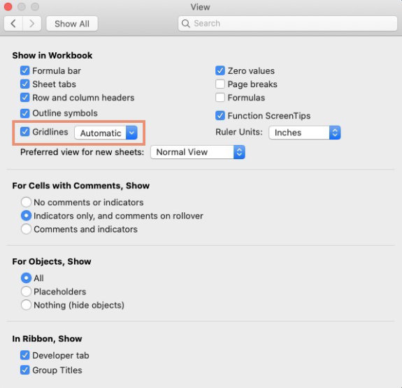
5. Click the box next to Gridlines.
6. Choose the color you want your gridlines to be.

Note: If you leave the color on Automatic, you will see only the light grey gridlines.

Change the grid line color in Excel for Windows

Gridline colors in Excel for Windows are managed in Excel’s Options panel.

1. Open the File tab.

2. Near the bottom of the menu, open Options.

3. Open the Advanced tab.

4. Scroll down the Advanced Options panel until you reach the section labeled Display Options For This Worksheet.

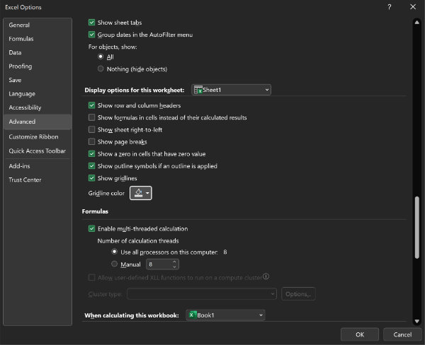
5. From the dropdown box, choose the worksheet that you are changing the gridlines on.

6. Choose a color.

Use borders for better visibility in Excel

Borders are not activated by default and are added as needed. Like gridline colors, they are managed on a sheet-by-sheet basis.

Borders cover or replace the grid lines and can be set to different weights and colors.

Borders will display even if the gridlines are disabled.

Apply borders in Excel

The easiest way to apply borders to your sheet is via the Borders button in the Font section of the Ribbon.

If you want to apply borders to the entire worksheet, select the entire sheet. You can do that using one of the following methods.

• Hit Command + A in Excel for Mac or Control + A in Excel for Windows.
• Click the small button in the corner to the left of column A and above Row 1. The button is divided diagonally into two colors – probably grey and white.

If you want to apply borders to just a section of the worksheet, drag your mouse to select the appropriate cells.

To apply borders to your selected cells:

Click the Borders button under the font selector in the Fonts section of the Ribbon.

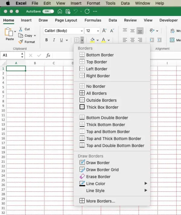
You will see a long list of border options. I suggest you choose your line style and color before you select the border. If you select the border first, your color and line styles may not apply properly.

The Format Cells panel in Excel

In Excel for Windows or Mac, if you click More Borders… at the bottom of the Borders button list, the Format Cells panel will open with the Borders tab pre-selected.

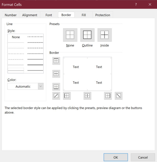
You can make adjustments to the borders you’ve already created, or create new borders.

Cell borders in Excel can also be created from the start through the Format Cells panel.

Open border settings in Excel

In Excel Windows or Mac, if you’re ever told to work with borders in the Format Cells panel, you can use one of the following methods.

Method one in Excel for Windows or Mac:

Right-click the cell, or selection of cells, that you want a border around.

1. Choose Format Cells…
2. Open the Border tab.

Method two in Excel for Windows or Mac:

1. Select the cells that you want a border around.
2. Open the Home tab.
3. Locate the Cells section of the ribbon.
4. Click the Format button. A menu will open.
5. Click Format Cells…
6. Open the Border tab.

Method three in Excel for Windows:

1. Select the cells that you want a border around.

2. In the lower right corner of the Fonts section, click the small button with an angled arrow in it.

3. Open the Border tab.

Method three in Excel for Mac:

1. Select the cells that you want a border around.
2. In the Format menu, select Cells….
3. Open the Border tab.

Any of the methods in this section will allow you to create new borders or change the borders you created in some other way.

Remember, the Format cells panel is the same panel you would see if you clicked More Borders… after clicking the Borders button in the Ribbon.

Use a custom style to quickly add borders in Excel

It takes a minute or two to create a custom cell style in Excel, but once you create it, you can apply dark borders to your cells with the click of a mouse button.

To create a custom cell style with darker borders:

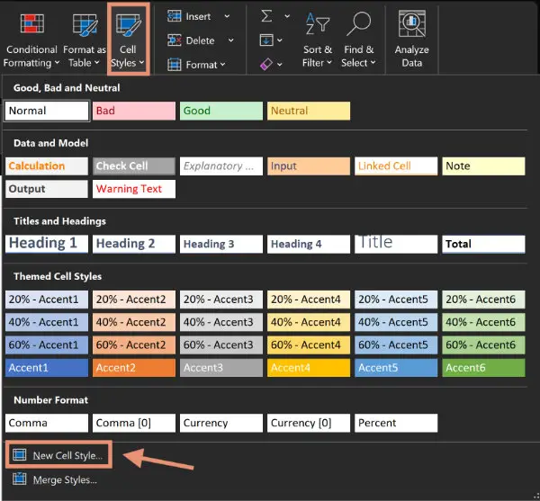
1. Open the Home tab.

2. In Excel for Windows, click the Custom Cell Styles button. In Excel for Mac, mouse over the bottom edge of the Styles section and click the small arrow.

3. At the bottom of the panel that opens, click New Cell Style...

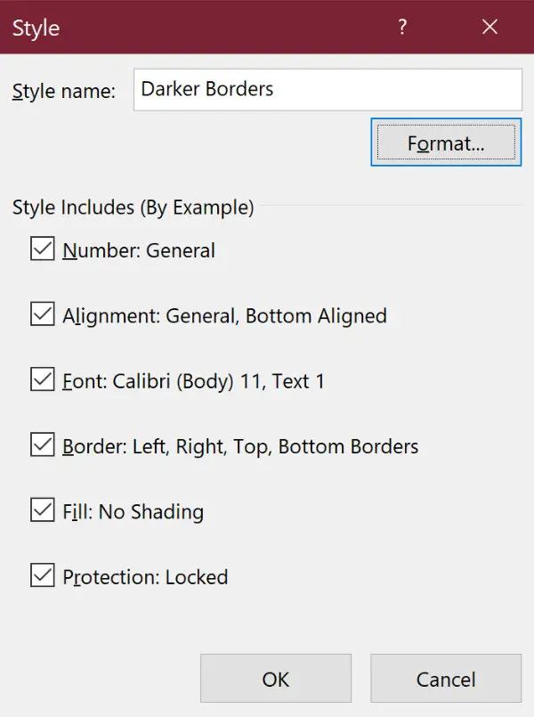
4. In the Style Name box, type in a descriptive name for your custom style.

5. In the bottom left corner on Macs or the top right corners in Windows, click Format…

6. The same Format Cells panel that we discussed earlier will open with the Border tab open.

7. For Line Color, choose any color other than Automatic.

8. Choose a Line Style, probably a heavier solid line.

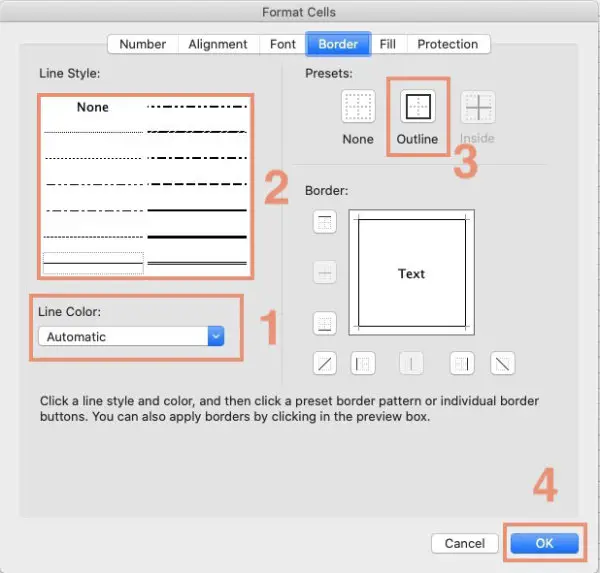
9. Under Presets in the right column, click Outline.

10. Click OK.

Now that you have a custom cell border set, you can very quickly set it by selecting the cells you want to have the bolder border. Then, click the button for the custom style you created. The button will be in the Styles section of the Home tab.

Use a template to create new sheets with custom styles

You can create a template that contains the new border styles. You can then base new workbooks on that template. When you start a new workbook, it automatically has those bolder borders.

To create a template with the styles you want, open a new blank workbook:

1. Make the styling changes that you want your future workbooks to include.
2. Under the File menu, click Save as Template…
3. Give your template a name, and click OK.

To use that template in new workbooks:

1. Go to File > New From Template….
2. Choose the newly styled blank template.

It is certainly not required, but I would recommend that you immediately rename and save your new workbook as an .XLSX file (File > Save As…).

Doing so can help you guard against filling your newly opened template and saving it later without changing it to a workbook. If that were to happen, the next time you open your template, you would find it full of the data that you typed in last time.

Save the new workbook under a new file name as an Excel Workbook (.xlxs). That will keep your template available as it was when you first opened it.

Other resources

If reading data in Excel sheets is difficult for you, you may also benefit from capitalizing text in Excel.

Microsoft’s documentation on other ways of using styles in Excel.